
Unlike hard sciences such as physics or chemistry, there is not a “correct” value of what a stock can be worth. Valuations depend on the inputs and assumptions one uses. We will go over several different valuation methods investors’ use. One of the most fundamental ways of valuing an asset is a method called a discounted cash-flow model, or a “DCF” model. Below is a description of this valuation method.
Background
The most basic way of valuing a company is assessing, how much “profit” a company generates. Assuming everything else equal, a company that generates more profits should be valued more than a company that generates less profit. To be able to put a fundamental value of a company, professional investors look at how much “profits” they believe the company will generate in the future and valuing what those values are today. The way most used method to do this analysis is called Discounted Cash Flow Model (“DCF”). It represents the sum of all future cash-flows a company generates discounting them back to today (adjusting it for the time value of money).
There are several steps to conduct when doing a DCF analysis of a company. We will go through each step below.
“Discounting” / Time Value of Money / Present Value
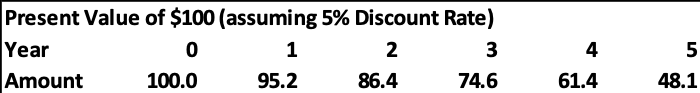
The concept of time value of money, or discounting “money” to today’s values. A good example of is assuming one has $100 today at a savings account which gives an annual interest of 5%. This $100 will be worth $105 in on years’ time. In year two it would be $110.3 ($105*1.05%). For each year that goes the money will grow with 5%. Below outlines how $100 grows over 5 years assuming 5% savings (interest) rate.

The same way money grows, as we can see above, with $100 growing to $127.6 in year 5 (assuming 5% growth rate), discounting money in the future to today will be the reverse. We are time adjusting the future value of money to the above example – the $127.6 in 5years is actually only worth $100 today (assumes 5% discount rate). In other words, the “present value” of $127.6 in 5 years is $100 assuming 5% discount rate. The equation is as follows;
Present Value = (Amount) / (1+r)^y
r= discount rate
y = number of years in the future.
Below, we can see that the “present value” of $100 in the future becomes less and less the further out in the future one goes. For example, the present value of $100 in 5years is only $48.1.
This discounting is used when valuing a company. One discounts back the future cash-flows of a company back to today. This would mean the “Present Value” of Future cash-flows. Another way of stating it is “discounted cash-flow”. The formula is:
Present Value of Cash Flows = (Cash Flow Year1)/ (1+r)1
+ (Cash Flow Year2)/ (1+r)2 + (Cash Flow Year3)/ (1+r)3
+….. (Cash Flow Yearx)/ (1+r)x
Free Cash Flow Definition
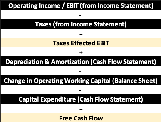
Now that we have explained the concept of discounting back. Next step for an investor is to assess what cash-flows we are going to discount back. Investors discount back Free-Cash-Flow (“FCF”). FCF is the amount of money that is left every year after the company has paid all operational expenses. It is calculated by taking a company’s Operating Income (EBIT), subtracting taxes, adding back Depreciation and Amortization, minus the Change in Operating Working Capital, Finally subtracting Capital Expenditures for each year.
All the historical numbers for “Free Cash Flow” (FCF) can be found in all listed companies public filings. But for our purposes to value the company one needs to discount back future Free Cash Flows into present value. To be able to do so we need to project future cash flows. There are various ways one can do this, and sometime this differs between various industries. We have chosen to show a general example below.
Projecting Future Free Cash-Flows
To be able to project all the various components of an FCF we need to make assumptions about the various input parts. Again there are several various steps which we will go through.
Arriving at future Operating Income (EBIT)

To arrive at Operating Income (EBIT) we need to make various assumptions for different income statement lines.
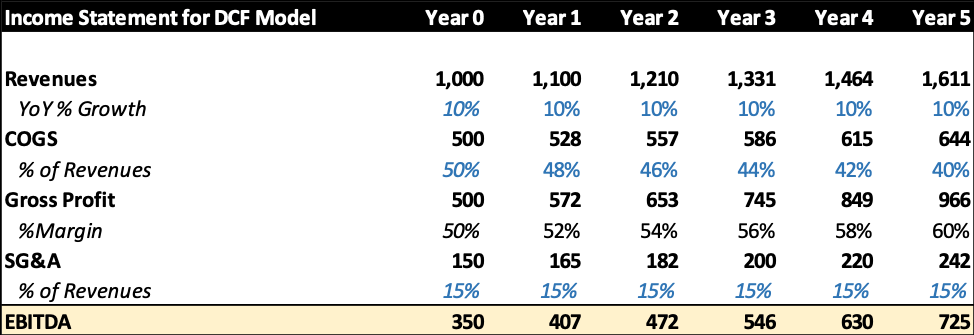
Revenues: This is the top line of the business. It is the company’s sales. Usually, professional investors assume a certain growth rate for revenues, based on the due-diligence they have done. This can be taking managements own projections, looking at peers and competitors, going through other analysts’ projections or for that matter their own assessment based on various factors. For our example, we will assume that revenues grow 10% yearly going forward.
Cost of Goods Sold (COGS): This is basically what it actually costs to build/generate the revenues. Often analysts assume this to be a % of sales that improves (decreases) over time. The assumption behind this is that as the company grows, economies of scale will start playing a larger factor and the company will become more efficient when comes to costs.
Selling, General, & Administrative (SG&A): This line item cost is assumed to be fairly stable as % of revenues over time. For example, a company would need to expand its advertising as revenues grow and so forth. On the flip-side, there is a business that SG&A amount increases less/stays fixed as for example a company might not need to do that much new advertising as it grows. These are assumptions that differ for each company or industry and how each investor analyses them. For our example, we are going to assume it is a constant 15% of sales.
Taking our Revenues, subtracting COGS and SG&A will give us EBITDA which will be used as part of the input for our FCF for our Discounted Cash Flow Model (DCF Model)
Example
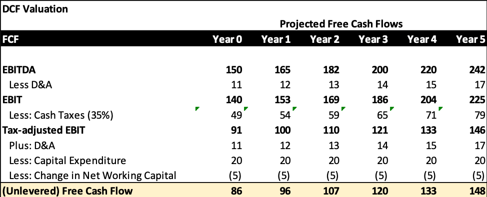
Depreciation & Amortization: Depreciation and Amortization (D&A) are both “non-cash” expenses. This means even though they are shown on the income statement, no actual cash was actually spent. One can see it as the expense item for capital expenditure (see below) that was spent in prior years. Hence to calculate “true” free-cash-flow one needs to add back D&A for the year. Often one assumes it to be a constant % of sales. For our example, we assume 7%
Capital Expenditure: Capital Expenditure is what the company spend on let say building a building or buying machinery. It is, in essence, the cash money spent on buying something that will help generate revenues in the future. As D&A is added back for the “true” FCF, the capital expenditure must be subtracted out as it does not appear in the income statement.
Building Free Cash Flow for DCF model/valuation
Next steps to build our FCF for our DCF model is to calculate the Free Cash Flow (Unlevered Free Cash Flow). Below are the steps that need to be taken.
Tax-adjusted (effected) EBIT: To calculate tax-adjusted EBIT, one needs to subtract D&A from EBITDA. As D&A is an expense for tax-purposes it needs to be subtracted from EBITDA. D&A will, later on, be added back for our calculations as it a “non-cash” expense
Tax Rate: This is often assumed to be the corporate tax-rate the company would pay. We assume 30% for our example
Depreciation & Amortization (D&A): As mentioned above D&A is added back because it is a non-cash expense.
Capital Expenditure: As Capital Expenditure is a cash-expense it needs to be subtracted out. It is the capital that is spent on various types of machinery that will support growth in the future. Usually deep in the future, as the company has reached “steady state”, Capital Expenditure and D&A tend to converge.
Change in Operating Working Capital (OWC): This represents the annual change of in current assets minus current liabilities on the balance sheet (note it excludes cash and cash-like items and debt).
All of this finally helps us derive FCF;
FCF = Tax Adjusted EBIT + D&A – Capital Expenditure – Change in OWC
Discounting Free Cash Flow Numbers
As part of the analysis, we have been able to calculate Free Cash Flow for the business for 5 years ahead. We need now to calculate the “Present Value”, or more correctly the net present value of all these future cash-flow to get the true value. We will then discount all the years FCF to current day.
As part of this analysis, the discount-rate is an important factor. For now, we will use a 5% discount rate. We later on further go into how to calculate discount-rate for each situation.
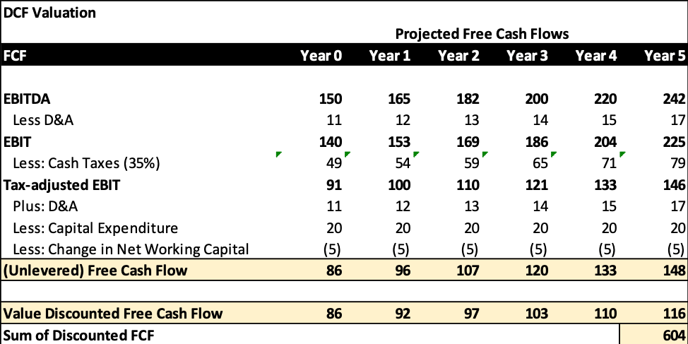
Based on our example with 5% discount rate, the total discounted value of FCF for the 5 years of our company is $604. Before we can reach the total value of our company, we also need to include the “Terminal Value” of our company.
Terminal Value
Terminal Value is the value of the company (in this instance FCF) that are after our projected period. In this example, our company will generate FCF post the 5 years we have made projected. We need to add the value of the all the future years FCF. The mechanism for this valuation calculation is called “Terminal Value”.
The way one calculates terminal value is through the something called the “The Perpetuity Method”. This method assumes that FCF will grow at a certain set constant rate into perpetuity. Often the growth-rate that is assumed in perpetuity is something at or very close to general GDP growth rate. Using higher growth rate assumptions can be faulty, as no company in the world into infinity grow higher than the general economic growth rate. If one assumes much higher growth rate than the GDP growth, not only will the valuation lose its foundation in reality, but also it assumes that the company eventually will be bigger than everything else in the world.

The process of calculating the terminal value through the perpetuity method is as follows.
- Assume and apply what one believes its long-term growth rate for FCF. We will assume GDP growth rate (g).
- Calculate terminal value by taking the FCF for the last projection year (for us year 5) * (1+ perpetual growth rate). Then one divides the result by taking the discount rate (r) and subtracting the assumed long-term growth rate.
Formula is: Terminal Value = FCFx * (1+g) / (r – g)
FCFx = Last projected year (period) of FCF for the company
g = the perpetual growth rate (often assumed GDP growth rate)
r = the discount rate (we used 5% in our examples so far). R is often calculated through something called the WACC calculation which we will address later in this piece.
For our example – for now, assume g of 2% and r is 5%. This would give Terminal Value as follows:
$5,030 = $148* (1+0.02) / (0.05-0.02)
We are getting very high Terminal Value compared to the discounted sum of our first 5 years of projections due to rather “low” discount rate (r). Often this rate is substantially higher than 5%.
To have a more accurate valuation, one needs to in more detail calculate the discount rate (r). We will demonstrate how this is done for each company/situation/project.
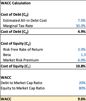
Weighted Cost of Capital (WACC)
The proper discount rate a professional investor uses when doing a DCF model is called “WACC”. In short, the WACC rate is the required rate of return for investors of investing in this business/company. In other words, the minimum rate of return an investor would need to invest in this specific company.
WACC is calculated as follows:
WACC = (CE *[(Equity / (Debt + Equity)]) + (CD *(1-Marginal Tax-rate)
*[Debt / (Debt + Equity)])
CE = Cost of Equity. CE = Crf + b × RP, where Crf equals the Risk Free Rate, b equals the levered (Equity) Beta for the company, and RP equals the Equity Market Risk Premium. The Beta and Risk Premium are calculated using the Capital Asset Pricing Model (CAPM). We are not going too much into detail for the background for CAPM model. Below is a brief explanation of the equation and various variables.
- Risk-Free-rate: This is often whatever the government say 10-year fund rate is. For our example, we are going to use 3%.
- Beta: Is the measure of a stock’s sensitivity of returns to changes in the market. It is a measure of systematic risk. A beta of 1 means company/stock is as “risky” as general market. A beta >1 means higher risk than the market and a beta <1 means safer. For our example, we are going to use a Beta of 1.3
- Equity Market Risk Premium (RP): RP = RMarket – C RMarket is the expected market return. We are going to use 9% in our example as that has is close what S&P500 have generated over the years.
CD = Cost of Debt. This is the weighted average of interest rates paid on the company’s outstanding debt. In WACC calculations, Cost of Debt is taken after taxes—i.e., it is multiplied by (1 – Tax-rate). This is due to the fact that Interest Expense on Debt is (most often) tax-deductible, thereby creating a tax shield which adds value to the company. This is represented in the DCF framework by reducing the Cost of Debt component of WACC, resulting in a lower discount rate for the company’s FCF, and therefore a higher valuation for the company.
Equity = Market Value of Equity, i.e., Market Capitalization.
Debt = Book Value of the company’s Debt.
Marginal Tax Rate = This rate can be different from the Effective Tax Rate used to determine Tax Expense based on EBIT.
All of this gives us the WACC-rate for our example. Which is 9.6%.
DCF Valuation of Company
Now that we have the WACC rate, we can apply this to our DCF Valuation, using this discount-rate both for the discounted value of our 5 year projected FCF but also for the Terminal Value.
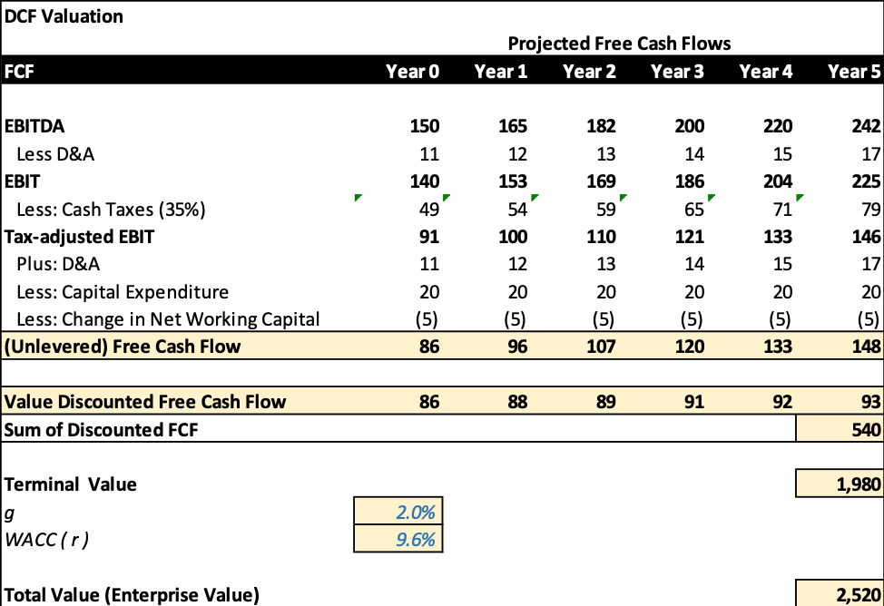
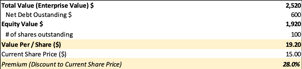
We now have the total DCF value for our company. This value is also known as the Enterprise Value.
To calculate the actual equity value and value per share we need to conduct two more steps.
- We need to remove the total net-debt (total debt – cash and cash equivalents) the company have outstanding from the Enterprise Value. This gives use Equity Value
- We need to then divide the Equity Value by total number of shares outstanding to calculate value per share
We can then compare the value from our DCF valuation to where the share price, if it is a listed stock, is trading. It will let us know if we with our DCF valuation value the stock higher/lower than the market does. In our example, using dummy numbers – our DCF valuation is at a 28% premium to where we this fictional stock is trading.
Pros and Cons of DCF Valuation
The pros with a DCF valuation is that it is based on a scientific method based on actual cash-flows of the company. The cons are that the valuation is completely based on the inputs we put in. Everything from our assumptions for revenue growth rates, to margins to discounts rates. All of these are more of an art than a science. If one as an investor is wrong on future cash-flows, then it does not matter how good rest of the analysis is, it will give us an incorrect valuation. Hence, professional investors and analysts spend a substantial amount of time conducting due diligence on various assumptions they make.
Best way to “mitigate” for all of this is to give oneself a “margin of safety”. In other words, making sure the potential upside we can calculate from our DCF valuation is substantially higher than the current share price in case we are wrong on one or several of our assumptions.